Comparison to Christensen et al. 2018
Renata Diaz, Juniper Simonis, and Hao Ye
Source:vignettes/paper-comparison.Rmd
paper-comparison.RmdIntroduction
This document provides a side-by-side comparison of LDATS (version 0.2.7) results with analysis from Christensen et al. 2018. Due to the size and duration of model runs, we use pre-generated model output from the LDATS-replications repo.
Summary
| Step | Changes from Christensen et al 2018 to LDATS
|
Effect on comparison | Recommendations for future users |
|---|---|---|---|
| Data | Paper adjusts abundances according to unit effort, while LDATS uses raw capture numbers. |
None: run comparison using adjusted data | Use raw, unweighted abundances. |
| LDA model selection | Paper conservatively overestimated the number of parameters for calculating AIC for model selection. LDATS calculates AIC appropriately. |
Paper LDA selects 4 topics, while LDATS finds 6. Compare all combinations of paper and LDATS LDA models and changepoint models |
Use LDATS AIC calculation. |
| Changepoint model document weights | Paper weighted all sampling periods equally regardless of abundance. LDATS by default weights the information from each sampling period according to the number of individuals captured (i.e. the amount of information gleaned about the underlying community composition). |
None; use weights = NULL to set all weights equal to 1 for LDATS |
Weight sampling periods according to abundance |
| Overall LDA + changepoint results | All combinations of LDA + changepoint model find 4 changepoints at approximately the same time steps | Choice of LDA model has more of an effect than choice of changepoint model |
LDATS reflects best practices, but the paper methods will produce qualitatively similar results. |
Setup
LDATS Installation
To obtain the most recent version of LDATS, install the most recent version from GitHub:
Load in the LDATS package.
To run the analyses here, you will also need to download dplyr, gridExtra, multipanel, RColorBrewer, RCurl, and reshape2 as the manuscript’s code relies on these packages.
Running the Models
Because both the Latent Dirichlet Allocation (LDA) and time series components of the analysis can take a long time to run (especially with the settings above for the number of seeds and iterations), we will use pre-generated model outputs and turn off certain code chunks that run the models using a global rmarkdown parameter, run_models = FALSE.
To change this functionality, you can re-render this file with:
Download Analysis Scripts and Data Files
We’re going to download analysis scripts, data files, and model objects, so we use a temporary location for storage:
To replicate the Christensen et al. 2018 analysis, we download some of the original scripts & data files from Extreme-events-LDA repo, as well as some raw data files from the PortalData repo, which are stored in the LDATS-replications repo:
Main Analysis Scripts:
-
rodent_LDA_analysis.R- main script for analyzing rodent community change using LDA
-
rodent_data_for_LDA.R- contains a function that creates the rodent data table used in analyses
-
AIC_model_selection.R- contains functions for calculating AIC for different candidate LDA models
-
changepointmodel.r- contains change-point model code
-
LDA-distance.R- function for computing Hellinger distance analyses
Data:
-
Rodent_table_dat.csv- table of rodent data, created by rodent_data_for_LDA.R
-
moon_dates.csv- table of census dates (downloaded from the PortalData repository)
-
Portal_rodent_trapping.csv- table of trapping effort (downloaded from the PortalData repository)
-
paper_dat.csv- rodent data table from Christensen et al. 2018
-
paper_dates.csv- dates used in Christensen et al. 2018
-
paper_covariates.csv- table of dates and covariate data
Figure scripts:
LDA_figure_scripts.R- contains functions for making main plots in manuscript (Fig 1). Called from rodent_LDA_analysis.R
test_file <- file.path(vignette_files, "scripts", "rodent_LDA_analysis.r")

if (!file.exists(test_file)){

  # scripts
  dir.create(file.path(vignette_files, "scripts"), showWarnings = FALSE)
  github_path <- "https://raw.githubusercontent.com/weecology/LDATS-replications/master/scripts/"
  files_to_download <- c("rodent_LDA_analysis.r", "rodent_data_for_LDA.r",
                         "AIC_model_selection.R", "changepointmodel.r",
                         "LDA-distance.R", "LDA_figure_scripts.R")

  for (file in files_to_download)  {
    download.file(url = paste0(github_path, file),
                  destfile = file.path(vignette_files, "scripts", file))
  }


  # data
  dir.create(file.path(vignette_files, "data"), showWarnings = FALSE)
  github_path <- "https://raw.githubusercontent.com/weecology/LDATS-replications/master/data/"
  files_to_download <- c("moon_dates.csv", "Portal_rodent_trapping.csv",
                         "Rodent_table_dat.csv", "paper_dat.csv",
                         "paper_dates.csv", "paper_covariates.csv")

  for (file in files_to_download)  {
    download.file(url = paste0(github_path, file),
                  destfile = file.path(vignette_files, "data", file))
  }
}
Download Model Outputs
We also have pre-generated model outputs that we download from the LDATS-replications repo:
LDA models:
-
ldats_ldamodel.RDS- the best LDA model as selected by LDATS
-
paper_ldamodel.RDS- the best LDA model as selected by the Christensen et al. analysis
Changepoint outputs:
-
ldats_ldats.RDS,ldats_ldats_cpt.RDS,ldats_ldats_cpt_dates.RDS- the posterior distribution, count, and dates of changepoints, using the LDATS LDA model and the LDATS changepoint selection
-
ldats_paper.RDS,ldats_paper_cpt.RDS, `ldats_paper_cpt_dates.RDS- the posterior distribution, count, and dates of changepoints, using the LDATS LDA model and the paper’s changepoint selection
-
paper_ldats.RDS,paper_ldats_cpt.RDS, `paper_ldats_cpt_dates.RDS- the posterior distribution, count, and dates of changepoints, using the paper LDA model and the LDATS changepoint selection
-
paper_paper.RDS,paper_paper_cpt.RDS, `paper_paper_cpt_dates.RDS- the posterior distribution, count, and dates of changepoints, using the paper LDA model and the paper’s changepoint selection
-
cpt_dates.RDS- summary table of changepoint results across models
Figures
-
lda_distances.png- figure showing the variance in the topics identified by the paper’s LDA model code
-
paper_paper_cpt_plot.png- figure showing the time series results for the paper analysis of the paper LDA
-
ldats_paper_cpt_plot.png- figure showing the time series results for the paper analysis of the LDATS LDA
-
annual_hist.RDS- function for making histogram of change points over years
test_file <- file.path(vignette_files, "output", "ldats_ldamodel.RDS")

if (!file.exists(test_file)){

  dir.create(file.path(vignette_files, "output"), showWarnings = FALSE)
  github_path <- "https://raw.githubusercontent.com/weecology/LDATS-replications/master/output/"
  files_to_download <- c("ldats_ldamodel.RDS", "paper_ldamodel.RDS",
                         "ldats_ldats.RDS", "ldats_paper.RDS",
                         "paper_ldats.RDS", "paper_paper.RDS",
                         "ldats_rodents_adjusted.RDS", "rodents.RDS",
                         "ldats_paper_cpt.RDS", "ldats_paper_cpt_dates.RDS",
                         "ldats_ldats_cpt.RDS", "ldats_ldats_cpt_dates.RDS",
                         "paper_paper_cpt.RDS", "paper_paper_cpt_dates.RDS",
                         "paper_ldats_cpt.RDS", "paper_ldats_cpt_dates.RDS",
                         "annual_hist.RDS", "cpt_dates.RDS",
                         "lda_distances.png", "paper_paper_cpt_plot.png",
                         "ldats_paper_cpt_plot.png")

  for (file in files_to_download){
    download.file(url = paste0(github_path, file),
                  destfile = file.path(vignette_files, "output", file),
                  mode = "wb")
  }
}
Data Comparison
The dataset of Portal rodents on control plots is included in the LDATS package:
data(rodents)

head(rodents[[1]])
#>   BA DM DO DS NA. OL OT PB PE PF PH PI PL PM PP RF RM RO SF SH SO
#> 1  0 13  0  2   2  0  0  0  1  1  0  0  0  0  3  0  0  0  0  0  0
#> 2  0 20  1  3   2  0  0  0  0  4  0  0  0  0  2  0  0  0  0  0  0
#> 3  0 21  0  8   4  0  0  0  1  2  0  0  0  0  1  0  0  0  0  0  0
#> 4  0 21  3 12   4  2  3  0  1  1  0  0  0  0  0  0  0  0  0  0  0
#> 5  0 16  1  9   5  2  1  0  0  2  0  0  0  0  0  0  1  0  0  0  0
#> 6  0 17  1 13   5  1  5  0  0  3  0  0  0  0  0  0  0  0  0  0  0
We can compare this against the data used in Christensen et al:
# parameters for subsetting the full Portal rodents data
periods <- 1:436
control_plots <- c(2, 4, 8, 11, 12, 14, 17, 22)
species_list <- c("BA", "DM", "DO", "DS", "NA", "OL", "OT", "PB", "PE", "PF",
                  "PH", "PI", "PL", "PM", "PP", "RF", "RM", "RO", "SF", "SH", "SO")

source(file.path(vignette_files, "scripts", "rodent_data_for_LDA.r"))

# assemble `paper_dat`, the data from Christensen et al. 2018
paper_dat <- create_rodent_table(period_first = min(periods),
                                 period_last = max(periods),
                                 selected_plots = control_plots,
                                 selected_species = species_list)

# assemble `paper_covariates`, the associated dates and covariate data
moondat <- read.csv(file.path(vignette_files, "data", "moon_dates.csv"), stringsAsFactors = F)

paper_dates <- moondat %>%
  dplyr::filter(period %>% dplyr::between(min(periods), max(periods))) %>%
  dplyr::pull(censusdate) %>%
  as.Date()

paper_covariates <- data.frame(
  index = seq_along(paper_dates),
  date = paper_dates,
  year_continuous = lubridate::decimal_date(paper_dates)) %>%
  dplyr::mutate(
    sin_year = sin(year_continuous * 2 * pi),
    cos_year = cos(year_continuous * 2 * pi)
  )
Compare the data from Christensen et al. with the included data in LDATS
There are 16 rows where the data included in LDATS differs from the paper data. This is because the LDATS data is not adjusted to account for trapping effort, while the paper data is, by dividing all census counts by the actual number of plots trapped and multiplying by 8 to account for incompletely-trapped censuses.
To confirm this, refer to lines 36-46 in rodent_data_for_LDA.r:
  # retrieve data on number of plots trapped per month
  trap_table = read.csv('https://raw.githubusercontent.com/weecology/PortalData/master/Rodents/Portal_rodent_trapping.csv')
  trap_table_controls = filter(trap_table, plot %in% selected_plots)
  nplots_controls = aggregate(trap_table_controls$sampled,by=list(period = trap_table_controls$period),FUN=sum)

  # adjust species counts by number of plots trapped that month
  r_table_adjusted = as.data.frame.matrix(r_table)
  for (n in 1:436) {
    #divide by number of control plots actually trapped (should be 8) and multiply by 8 to estimate captures as if all plots were trapped
    r_table_adjusted[n,] = round(r_table_adjusted[n,]/nplots_controls$x[n]*8)
  }
We can run the same procedure on the LDATS data to verify that we obtain a data.frame that matches.
# get the trapping effort for each sample
trap_table <- read.csv(file.path(vignette_files, "data", "Portal_rodent_trapping.csv"))
trap_table_controls <- dplyr::filter(trap_table, plot %in% control_plots)
nplots_controls <- aggregate(trap_table_controls$sampled,
                            by = list(period = trap_table_controls$period),
                            FUN = sum)

# adjust species counts by number of plots trapped that month
#   divide by number of control plots actually trapped (should be 8) and
#   multiply by 8 to estimate captures as if all plots were trapped
ldats_rodents_adjusted <- as.data.frame.matrix(rodents[[1]])
ldats_rodents_adjusted[periods, ] <- round(ldats_rodents_adjusted[periods, ] / nplots_controls$x[periods] * 8)
Now we can compare the adjusted LDATS dataset with both the original ldats dataset and the dataset from the paper:
compare_raw <- rodents[[1]] == ldats_rodents_adjusted
length(which(rowSums(compare_raw) < ncol(compare_raw)))

compare_adjusted <- ldats_rodents_adjusted == paper_dat
length(which(rowSums(compare_adjusted) < ncol(compare_adjusted)))
Because the LDA procedure weights the information from documents (census periods) according to the number of words (rodents captured), we now believe it is most appropriate to run the LDA on unadjusted trapping data, and we recommend that users of LDATS do so. However, to maintain consistency with Christensen et al 2018, we will proceed using the adjusted rodent table in this vignette.
The LDATS rodent data comes with a document_covariate_table, which we will use later as the predictor variables for the changepoint models. In this table, time is expressed as new moon numbers. Later we will want to be able to interpret the results in terms of census dates. We will add a column to the document_covariate_table to convert new moon numbers to census dates. We will not reference this column in any of the formulas we pass to the changepoint models, so it will be ignored until we need it.
Identify community groups using LDA
While LDATS can run start-to-finish with LDATS::LDA_TS, here we will work through the process function-by-function to isolate differences with the paper. For a breakdown of the LDA_TS pipeline, see the codebase vignette.
First, we run the LDA models from LDATS to identify the number of topics:
ldats_ldas <- LDATS::LDA_set(document_term_table = rodents$document_term_table,
                             topics = 2:6, nseeds = nseeds)
ldats_ldamodel <- LDATS::select_LDA(LDA_models = ldats_ldas)[[1]]

saveRDS(ldats_ldamodel, file = file.path(vignette_files, "ldats_ldamodel.RDS"))
Second, we run the LDA models from Christensen et al. to do the same task:
source(file.path(vignette_files, "scripts", "AIC_model_selection.R"))
source(file.path(vignette_files, "scripts", "LDA-distance.R"))

# Some of the functions require the data to be stored in the `dat` variable
dat <- paper_dat

# Fit a bunch of LDA models with different seeds
# Only use even numbers for seeds because consecutive seeds give identical results
seeds <- 2 * seq(nseeds)

# repeat LDA model fit and AIC calculation with a bunch of different seeds to test robustness of the analysis
best_ntopic <- repeat_VEM(paper_dat,
                          seeds,
                          topic_min = 2,
                          topic_max = 6)
hist(best_ntopic$k, breaks = seq(from = 0.5, to = 9.5),
     xlab = "best # of topics", main = "")

# 2b. how different is species composition of 4 community-types when LDA is run with different seeds?
# ==================================================================
# get the best 100 seeds where 4 topics was the best LDA model
seeds_4topics <- best_ntopic %>%
  filter(k == 4) %>%
  arrange(aic) %>%
  head(min(100, nseeds)) %>%
  pull(SEED)

# choose seed with highest log likelihood for all following analyses
#    (also produces plot of community composition for "best" run compared to "worst")

png(file.path(vignette_files, "output", "lda_distances.png"), width = 800, height = 400)
dat <- paper_dat # calculate_LDA_distance has some required named variables
best_seed <- calculate_LDA_distance(paper_dat, seeds_4topics)
dev.off()
mean_dist <- unlist(best_seed)[2]
max_dist <- unlist(best_seed)[3]

# ==================================================================
# 3. run LDA model
# ==================================================================
ntopics <- 4
SEED <- unlist(best_seed)[1]  # For the paper, use seed 206
ldamodel <- LDA(paper_dat, ntopics, control = list(seed = SEED), method = "VEM")

saveRDS(ldamodel, file = file.path(vignette_files, "paper_ldamodel.RDS"))
Plots
To visualize the LDA assignment of species to topics, we load in the saved LDA models from previously:
ldamodel <- readRDS(file.path(vignette_files, "output", "paper_ldamodel.RDS"))
ldats_ldamodel <- readRDS(file.path(vignette_files, "output", "ldats_ldamodel.RDS"))
How the paper LDA model assigns species to topics:
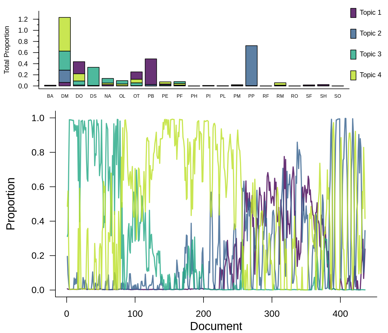
How the LDATS LDA model assigns species to topics:
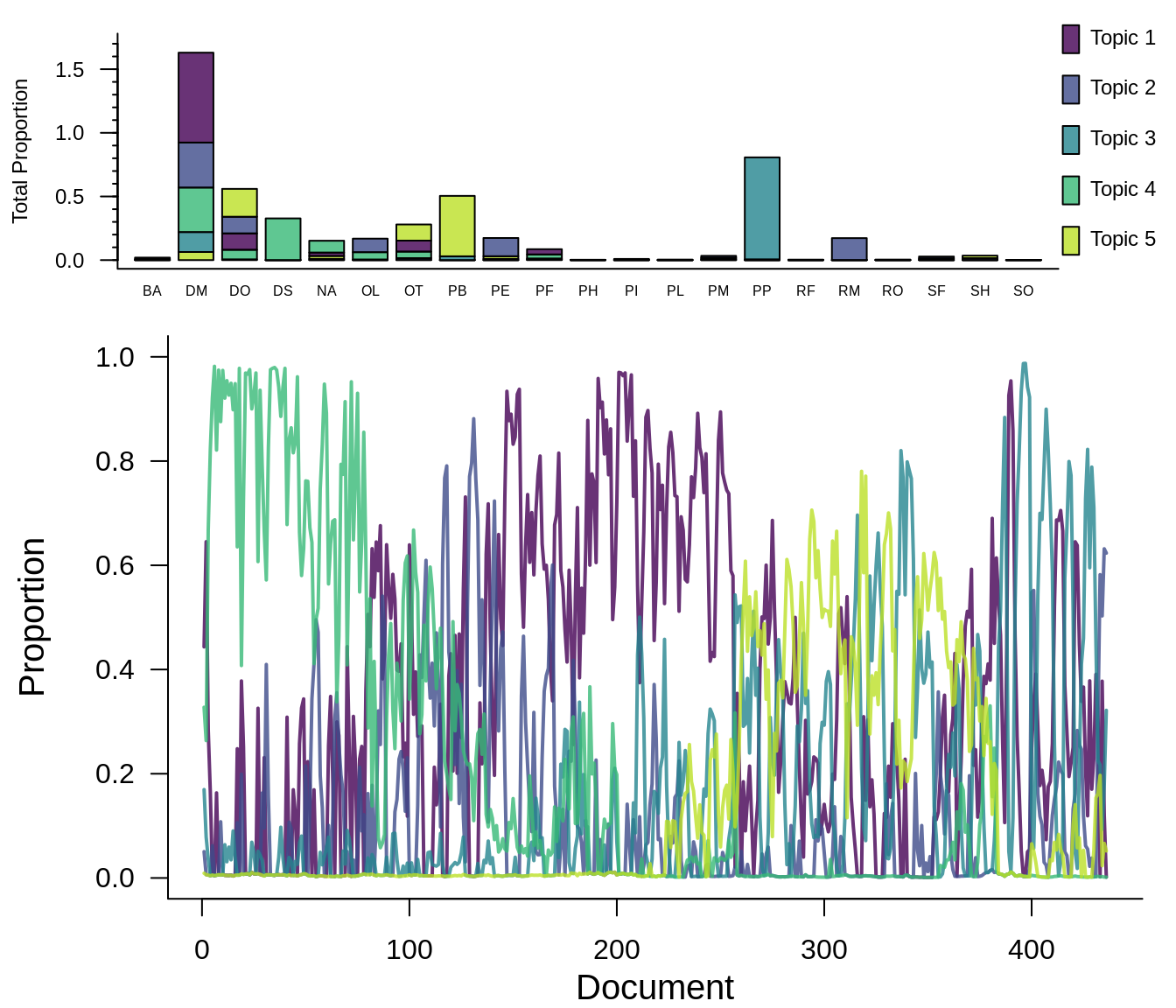
The paper method finds 4 topics and LDATS finds 6. This is because of an update to the model selection procedure. The paper conservatively overestimates the number of parameters (by counting all of the variational parameters) and therefore overpenalizes the AIC for models with more topics. Comparatively, the LDATS method now uses the number of parameters remaining after the variational approximation, as returned by the LDA object. For this vignette, we will compare the results from using both LDA models.
Changepoint models
We will compare four combinations of LDA + changepoint models:
- LDATS LDA + LDATS changepoint
- LDATS LDA + paper changepoint
- Paper LDA + LDATS changepoint
- Paper LDA + paper changepoint
Having divided the data to generate catch-per-effort, the paper changepoint model weighted all sample periods equally. In comparison, LDATS does not force an equal weighting, but assumes that as default, and can weight sample periods according to how many individuals were captured (controlled by the weights argument to LDA_TS, and easily calculated for a document-term matrix using document_term_weights. We now believe it is more appropriate to weight periods proportional to captures in the time series (despite the LDA function returning only proportions of each topic), and this is what we recommend for LDATS users. For the purposes of comparison, however, we will continue set all weights = 1 for both changepoint models. For an example of LDATS run with proportional weights, see the rodents vignette.
Running paper changepoint models
We define a few helper functions for running the changepoints model of Christensen et al. and processing the output to obtain the dates:
#### Run changepoint ####
source(file.path(vignette_files, "scripts", "changepointmodel.r"))

find_changepoints <- function(lda_model, paper_covariates, n_changepoints = 1:6){
  # set up parameters for model
  x <- dplyr::select(paper_covariates,
                     year_continuous,
                     sin_year,
                     cos_year)

  # run models with 1, 2, 3, 4, 5, 6 changepoints
  cpt_results <- data.frame(n_changepoints = n_changepoints)
  cpt_results$cpt_model <- lapply(cpt_results$n_changepoints,
                                  function(n_changepoints){
                                    changepoint_model(lda_model, x, n_changepoints, maxit = nit,
                                                      weights = rep(1, NROW(x)))
                                  })
  return(cpt_results)
}

# Among a selection of models with different # of changepoints,
#   - compute AIC
#   - select the model with the best AIC
#   - get the posterior distributions for the changepoints
select_cpt_model <- function(cpt_results, ntopics){
  # compute log likelihood as the mean deviance
  cpt_results$mean_deviances <- vapply(cpt_results$cpt_model,
                                       function(cpt_model) {mean(cpt_model$saved_lls)},
                                       0)

  # compute AIC = ( -2 * log likelihood) + 2 * (#parameters)
  cpt_results$AIC <- cpt_results$mean_deviances * -2 +
    2 * (3 * (ntopics - 1) * (cpt_results$n_changepoints + 1) +
           (cpt_results$n_changepoints))

  # select the best model
  cpt <- cpt_results$cpt_model[[which.min(cpt_results$AIC)]]
  return(cpt)
}

# transform the output from `compute_cpt` and match up the time indices with
#   dates from the original data
get_dates <- function(cpt, covariates = paper_covariates){
  cpt$saved[,1,] %>%
    t() %>%
    as.data.frame() %>%
    reshape::melt() %>%
    dplyr::left_join(covariates, by = c("value" = "index"))
}
LDATS LDA and paper changepoint
Run the Christensen et al. time series model to identify changepoints on the LDA topics selected by LDATS:
ldats_paper_results <- find_changepoints(ldats_ldamodel, paper_covariates)

saveRDS(ldats_paper_results, file = file.path(vignette_files, "output", "ldats_paper.RDS"))
Extract the dates of the changepoints:
Paper LDA and paper changepoint
Run the Christensen et al. time series model to identify changepoints on the LDA topics selected by Christensen et al.:
paper_paper_results <- find_changepoints(ldamodel, paper_covariates)

saveRDS(paper_paper_results, file = file.path(vignette_files, "paper_paper.RDS"))
Extract the dates of the changepoints:
Running LDATS changepoint models
LDATS LDA and LDATS changepoint
Run the LDATS time series model to identify changepoints on the LDA topics selected by LDATS:
ldats_ldats_results <- TS_on_LDA(LDA_models = ldats_ldamodel,
                                 document_covariate_table = rodents$document_covariate_table,
                                 formulas = ~ sin_year + cos_year,
                                 nchangepoints = 1:6,
                                 timename = "newmoon",
                                 weights = NULL,
                                 control = list(nit = nit))

saveRDS(ldats_ldats_results, file = file.path(vignette_files, "output", "ldats_ldats.RDS"))
Unlike the paper changepoint model, LDATS can recognize that sampling periods may not be equidistant, and can place changepoint estimates at new moons if they fall between nonconsecutive sampling periods. We can estimate the dates corresponding to those new moons, extrapolating from the census dates for adjacent census periods.
# make the full sequence of possible newmoon values
full_index <- seq(min(rodents$document_covariate_table$newmoon),
                  max(rodents$document_covariate_table$newmoon))

# generate a lookup table with dates for the newmoons, using `approx` to
#   linearly interpolate the missing values
ldats_dates <- approx(rodents$document_covariate_table$newmoon,
                     as.Date(rodents$document_covariate_table$date),
                     full_index) %>%
  as.data.frame() %>%
  mutate(index = x,
         date = as.Date(y, origin = "1970-01-01")) %>%
  select(index, date)
Select the best time series model and extract the dates of the changepoints:
Paper LDA and LDATS changepoint
Run the LDATS time series model to identify changepoints on the LDA topics selected by Christensen et al.:
paper_ldats_results <- TS_on_LDA(LDA_models = ldamodel,
                             document_covariate_table = rodents$document_covariate_table,
                             formulas = ~ sin_year + cos_year,
                             nchangepoints = 1:6,

                             timename = "newmoon",
                             weights = NULL,
                             control = list(nit = nit))


saveRDS(paper_ldats_results, file = file.path(vignette_files, "output", "paper_ldats.RDS"))
Select the best time series model and extract the dates of the changepoints:
How many changepoints were identified?
nlevels(ldats_paper_cpt_dates$variable)
#> [1] 4
nlevels(paper_paper_cpt_dates$variable)
#> [1] 4
nlevels(ldats_ldats_cpt_dates$variable)
#> [1] 4
nlevels(paper_ldats_cpt_dates$variable)
#> [1] 4
All of the models find four changepoints.
Plot changepoint models
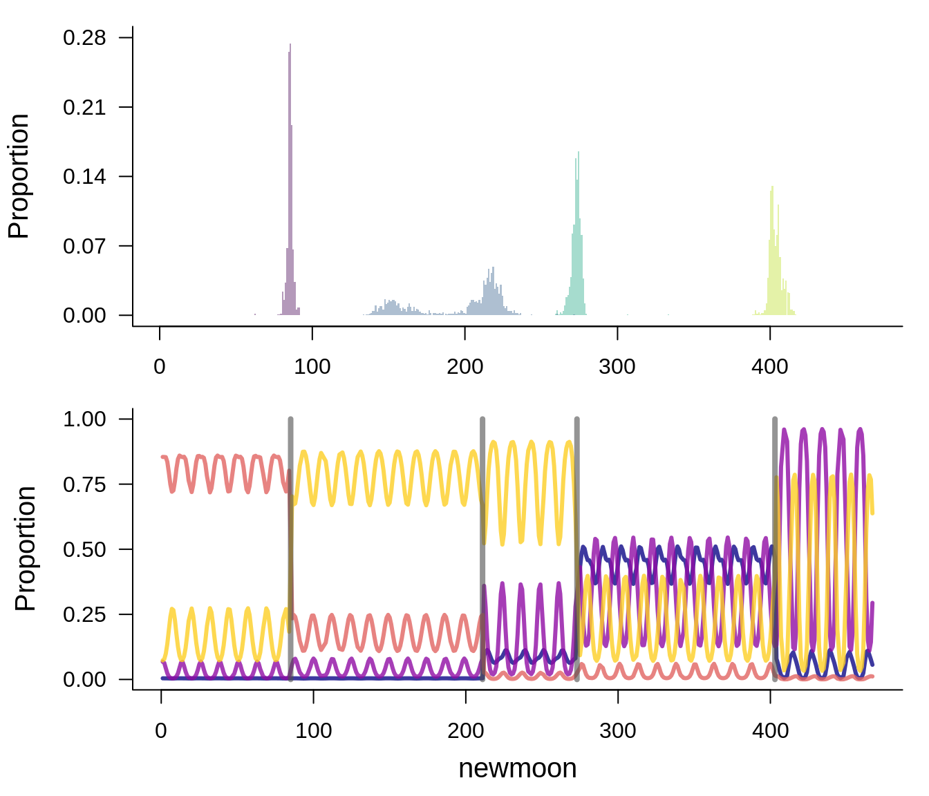
Paper LDA and paper changepoint
paper_cpts <- find_changepoint_location(paper_paper_cpt)
ntopics <- ldamodel@k

png(file.path(vignette_files, "output", "paper_paper_cpt_plot.png"), width = 800, height = 600)
get_ll_non_memoized_plot(ldamodel, paper_covariates, paper_cpts, make_plot = TRUE,
                                           weights = rep(1, NROW(paper_covariates)))
dev.off()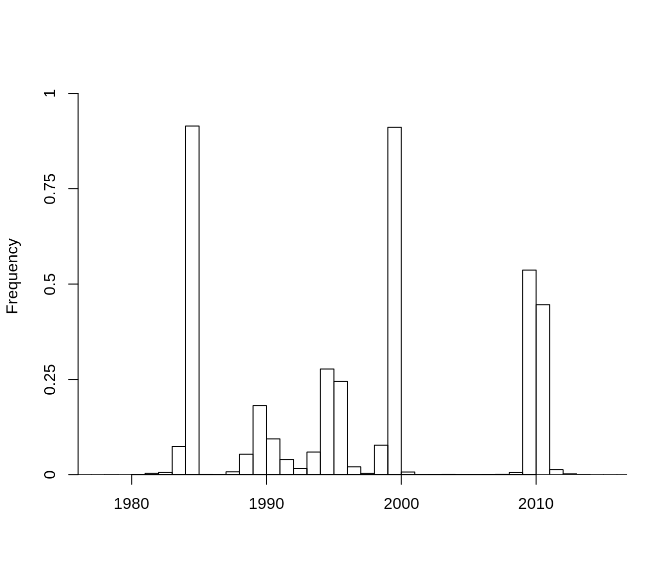

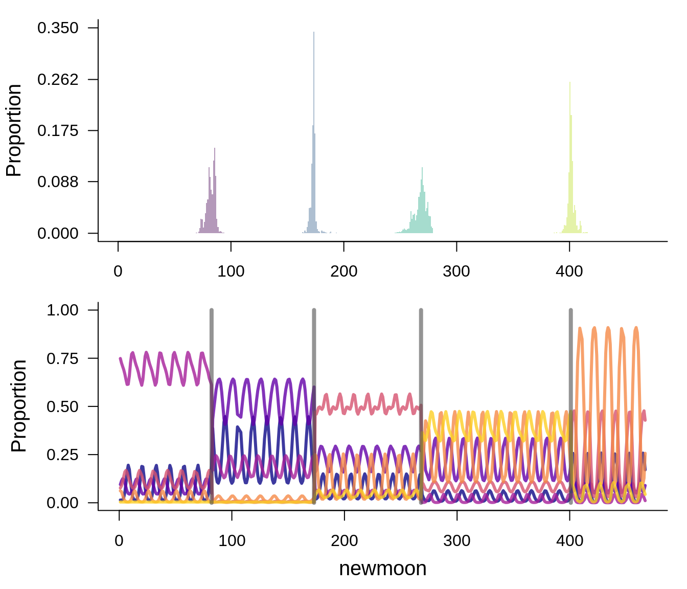
LDATS LDA and paper changepoint
ldats_cpts <- find_changepoint_location(ldats_paper_cpt)
ntopics <- ldats_ldamodel@k

png(file.path(vignette_files, "output", "ldats_paper_cpt_plot.png"), width = 800, height = 600)
get_ll_non_memoized_plot(ldats_ldamodel, paper_covariates, ldats_cpts, make_plot = TRUE,
                                           weights = rep(1, NROW(paper_covariates)))
dev.off()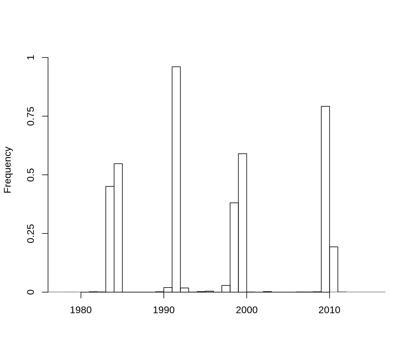

The results of the changepoint model appear robust to both choice of LDA model and choice of changepoint model.
Report changepoint dates
| changepoint | ldatsLDA_ldatsCPT | ldatsLDA_paperCPT | paperLDA_ldatsCPT | paperLDA_paperCPT |
|---|---|---|---|---|
| V1 | 1984-01-30 | 1984-01-11 | 1984-04-27 | 1984-01-11 |
| V2 | 1991-05-30 | 1991-05-29 | 1993-04-19 | 1991-05-29 |
| V3 | 1999-01-25 | 1998-12-21 | 1999-07-07 | 1998-12-21 |
| V4 | 2009-11-15 | 2009-09-29 | 2010-01-20 | 2009-09-29 |
The choice of LDA has more influence on the changepoint locations than the choice of changepoint model - probably because the LDATS LDA has 6 topics, and the paper LDA has 4. However, all of the models agree to within 6 months in most cases, and a year for the broader early 1990s changepoint.