LDATS Rodents Example
Renata Diaz and Juniper L. Simonis
Source:vignettes/rodents-example.Rmd
rodents-example.RmdThis vignette walks through an example of LDATS at the command line and was constructed using LDATS version 0.2.7 on 2020-03-19.
Installation
To obtain the most recent version of LDATS, install and load the most recent version from GitHub:
Data
For this vignette, we will be using rodent data from the control plots of the Portal Project, which come with the LDATS package (data(rodents)).
rodents contains two data tables, a document_term_table and a document_covariate_table.
The document_term_table is a matrix of species (term) counts by sampling period (document). Importantly, the document_term_table contains raw counts of individual rodent captures, not catch per unit effort. The LDA models operate on proportions and weight the information from each sampling period according to total catch (document size). Similarly, the TS models use the LDA compositional breakdown and weight the information from each period according to the total catch. We therefore give both models unadjusted data. The values in the document_term_table must be integers.
The document_covariate_table contains the covariates we would like to use for the time series models. In this case, we have a column for newmoon, which is the time step for each of our sampling periods. This column can include nonconsecutive time steps (i.e., 2, 4, 5) if sampling periods are skipped or at unequal intervals, but must be integer-conformable or a date. Although if a date, the assumption is that the timestep is 1 day, which is often not desired behavior. If there is no time column, LDATS will assume all time steps are equidistant. We also include columns sin_year and cos_year so we can account for seasonal dynamics.
data(rodents)
head(rodents$document_term_table, 10)
#>    BA DM DO DS NA. OL OT PB PE PF PH PI PL PM PP RF RM RO SF SH SO
#> 1   0 13  0  2   2  0  0  0  1  1  0  0  0  0  3  0  0  0  0  0  0
#> 2   0 20  1  3   2  0  0  0  0  4  0  0  0  0  2  0  0  0  0  0  0
#> 3   0 21  0  8   4  0  0  0  1  2  0  0  0  0  1  0  0  0  0  0  0
#> 4   0 21  3 12   4  2  3  0  1  1  0  0  0  0  0  0  0  0  0  0  0
#> 5   0 16  1  9   5  2  1  0  0  2  0  0  0  0  0  0  1  0  0  0  0
#> 6   0 17  1 13   5  1  5  0  0  3  0  0  0  0  0  0  0  0  0  0  0
#> 7   0 19  0  9   4  2  3  0  1  1  0  0  0  0  0  0  0  0  0  0  0
#> 8   0 15  0  9   2  1  2  0  1  2  0  0  0  0  0  0  0  0  0  0  0
#> 9   0 11  1 12   1  1  5  0  2  3  0  0  0  0  0  0  1  0  0  0  0
#> 10  0 14  1 15   1  0  0  0  0  0  0  0  0  0  0  0  0  0  0  0  0
head(rodents$document_covariate_table, 10)
#>    newmoon sin_year cos_year
#> 1        1  -0.2470  -0.9690
#> 2        2  -0.6808  -0.7325
#> 3        3  -0.9537  -0.3008
#> 4        4  -0.9813   0.1925
#> 5        5  -0.7583   0.6519
#> 6        6  -0.3537   0.9354
#> 7        7   0.1373   0.9905
#> 8        8   0.6085   0.7936
#> 9        9   0.9141   0.4054
#> 10      10   0.9951  -0.0988
Stage 1: LDA models
We use LDA_set() to run replicate LDA models (each with its own seed) with varying numbers of topics (2:5) and select_LDA() to select the best model.
We use the control argument to pass controls to the LDA function via a list. In this case, we can set quiet = TRUE to make the model run quietly.
lda_model_set <- LDA_set(document_term_table = rodents$document_term_table,
                         topics = c(2:5),
                         nseeds = 10,
                         control = list(quiet = TRUE))
If we do not pass any controls, by default, quiet = FALSE (here run with only 2:3 topics and 2 seeds, to keep output short):
lda_model_set2 <- LDA_set(document_term_table = rodents$document_term_table,
                         topics = c(2:3),
                         nseeds = 2)
LDA_set() returns a list of LDA models. We use select_LDA() to identify the best number of topics and choice of seed from our set of models. By default, we will choose models based on minimum AIC. To use different selection criteria, define the appropriate functions and specify them by passing list(measurer = [measurer function], selector = [max, min, etc]) to the control argument.
We can access the results of the model:
# Number of topics:
selected_lda_model[[1]]@k
#> [1] 5
# Topic composition of communities at each time step
# Columns are topics; rows are time steps
head(selected_lda_model[[1]]@gamma)
#> [,1] [,2] [,3] [,4] [,5]
#> [1,] 0.008303695 0.466475067 0.3431302 0.008585984 0.173505077
#> [2,] 0.005769837 0.663030049 0.2480563 0.005808044 0.077335746
#> [3,] 0.005008333 0.325407486 0.6280921 0.005095116 0.036397003
#> [4,] 0.003986846 0.183762181 0.8042557 0.004034794 0.003960483
#> [5,] 0.005016414 0.005116156 0.9210663 0.063795689 0.005005489
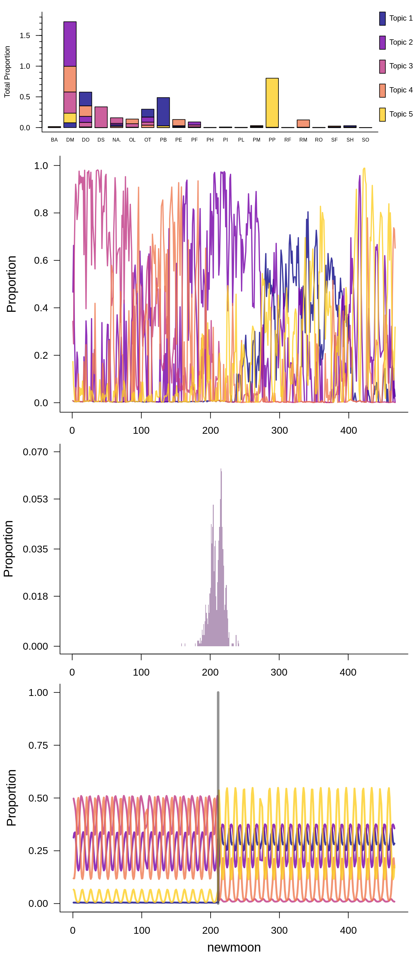
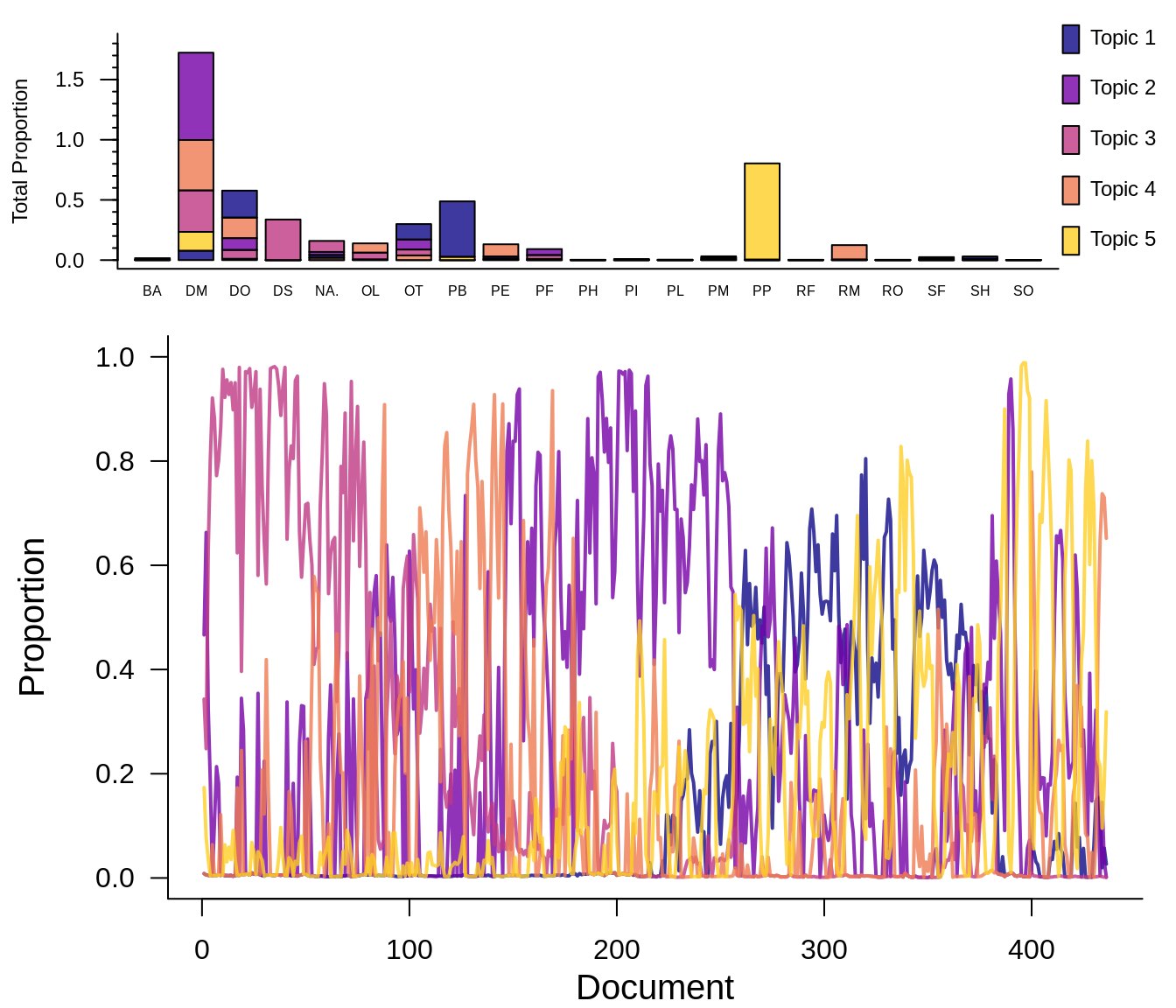
#> [6,] 0.004157612 0.105779863 0.8817614 0.004170617 0.004130473LDATS includes flexible plot functionality for LDAs and time series. The top panel illustrates topic composition by species, and the bottom panel shows the proportion of the community made up of each topic over time. For all the available plot options see ?plot.LDA_VEM.
Stage 2: TS changepoint models
We use TS_on_LDA() to run LDATS changepoint models with 0:6 changepoints, and then use select_TS() to find the best-fit model of these.
Here, TS_on_LDA() predicts the gamma (the proportion of the community made of up each topic) from our LDA model(s) as a function of sin_year and cos_year in the document_covariate_table. We use document_weights() to weight the information from each time step according to the total number of rodents captured at that time step.
changepoint_models <- TS_on_LDA(LDA_models = selected_lda_model,
                                document_covariate_table = rodents$document_covariate_table,
                                formulas = ~ sin_year + cos_year,
                                nchangepoints = c(0:1),
                                timename = "newmoon",
                                weights = document_weights(rodents$document_term_table),
                                control = list(nit = 1000))
We can adjust options (default settings can be seen using TS_control()) for both TS functions by passing a list to the control argument. For a full list see ?TS_control. Here we illustrate adjusting the number of ptMCMC iterations - the default is 10000, but it is convenient to use fewer iterations for code development.
Also, it is important to note that by default the TS functions take the name of the time-step column from the document_covariate_table to be "time". To pass a different column name, use the timename argument in TS_on_LDA().
select_TS() will identify the best-fit changepoint model of the models from TS_on_LDA(). As with select_LDA(), we can adjust the measurer and selector functions using the control argument list.
We can access the results of the selected changepoint model:
# Number of changepoints
selected_changepoint_model$nchangepoints
#> [1] 1
# Summary of timesteps (newmoon values) for each changepoint
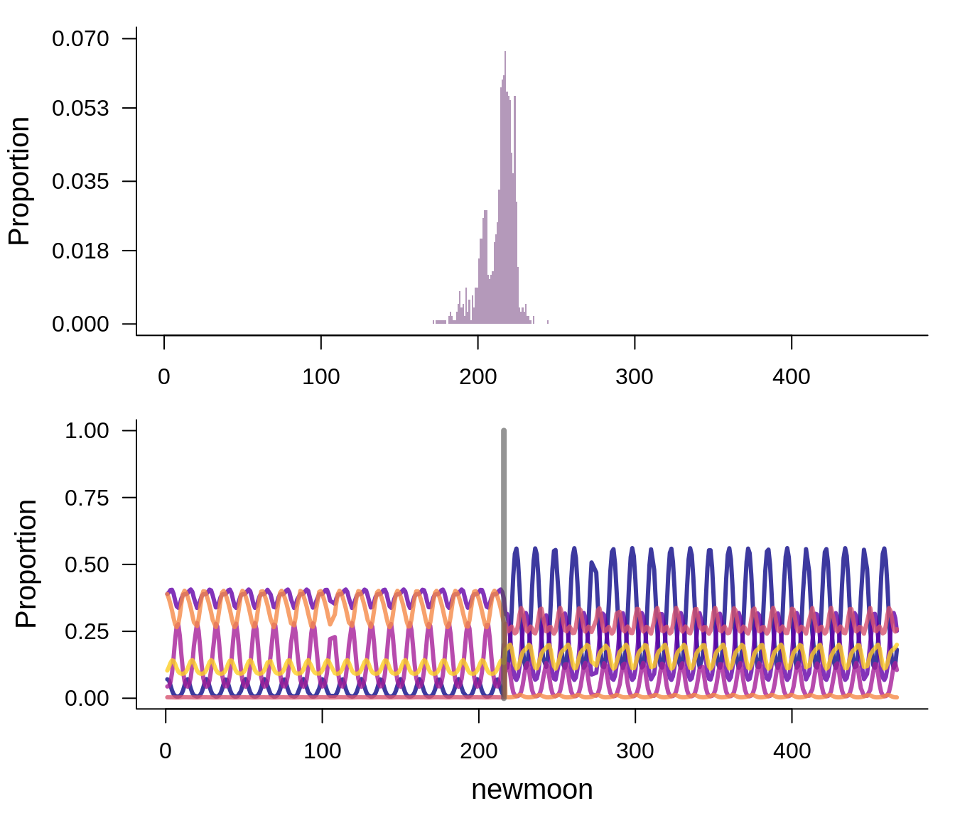
selected_changepoint_model$rho_summary
#> Mean Median Mode Lower_95% Upper_95% SD MCMCerr AC10
#> Changepoint_1 212.93 216 217 187 225 10.03 0.3172 0.0066
#> ESS
#> Changepoint_1 360.2996
# Raw estimates for timesteps for each changepoint
# Changepoints are columns
head(selected_changepoint_model$rhos)
#> [,1]
#> [1,] 220
#> [2,] 220
#> [3,] 218
#> [4,] 215
#> [5,] 213
#> [6,] 216LDATS will plot the results of a changepoint model:
Full analysis with LDA_TS
Finally, we can perform an entire LDATS analysis, including all of the above steps, using the LDA_TS() function and passing options to the LDA and TS functions as a list to the control argument. The default is for LDA_TS to weight the time series model based on the document sizes, so we do not need to tell it to do so.
lda_ts_results <- LDA_TS(data = rodents,
                         nseeds = 10,
                         topics = 2:5,
                         formulas = ~ sin_year + cos_year,
                         nchangepoints= 0:1,
                         timename = "newmoon",
                         control = list(nit = 1000))
LDA_TS() returns a list of all the model objects, and we can access their contents as above:
names(lda_ts_results)
#> [1] "LDA models"         "Selected LDA model" "TS models"
#> [4] "Selected TS model"

# Number of topics
lda_ts_results$`Selected LDA model`$k@k
#> [1] 5

# Number of changepoints
lda_ts_results$`Selected TS model`$nchangepoints
#> [1] 1

# Summary of changepoint locations
lda_ts_results$`Selected TS model`$rho_summary
#>                 Mean Median Mode Lower_95% Upper_95%  SD MCMCerr   AC10
#> Changepoint_1 209.26    211  215       190       225 9.7  0.3067 0.0104
#>                    ESS
#> Changepoint_1 380.3491
Finally, we can plot the LDA_TS results.